Everyday we deal with online platforms that use recommendation systems. There are different approaches to implement such systems and it depends on the product, the available data and more.
This post will mainly focus on collaborative filtering using embeddings as a way to learn about latent factors. I learned about this approach months ago from fast.ai Practical Deep Learning for Coders lessons. I also found out that StichFix wrote about the same concept in a blog post last year Understanding Latent Style.
Here will use the goodbooks-10k dataset, which contains " around six million ratings for ten thousand books". The post will explain the high-level concepts then it will show preliminary Keras models to demonstrate two methods in which we can use embeddings to represent our data. We will refer to the two methods as:
- Matrix factorization method
- Tabular data method
Note that the examples are for demo purposes and they are not intended to provide the best model. Also I am not aware of a benchmark for this dataset, so the comparison with other models is out of this post’s scope
Matrix Factorization, Latent Factors and Embeddings
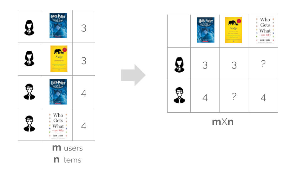
In a platform like goodreads, we see book recommendations based on the history of the user, similarities with other users or other signals collected about the user behavior. In practice, different signals and algorithms are usually merged to get better results. But let’s focus on one approach; item-based collaborative filtering. Using this approach, we learn about the similarities between the books from the ratings we already have. Starting with tabular data, the first step is to convert our table to a matrix with one row per user as shown in the following figure.
But what is the problem with that?
Usually we’ll have thousands of users and items, so this matrix will be very sparse with dimensions (mXn) .
What is the common solution?
To reduce the complexity of the problem, it is common to deal with lower-dimension matrices using matrix factorization. The idea is to represent each user/item by a compact vector representing the latent factors.
And How can embeddings help?
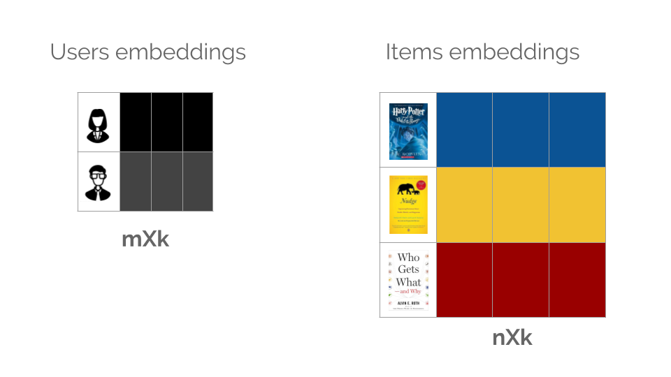
Instead of the traditional ways, we can use embedding layers and learn about the latent factors while training our neural network using the given ratings. As a result we will have:
- Users embedding (mXk)
- Items embedding (nXk)
Ideally, with a good model, users/items close to each other in the space should have similar characteristics.
Then we can use these matrices in two ways:
1- Matrix factorization method where we take these matrices, calculate the element-wise product of (mXk),(kXm) then add other fully connected layers.

2 - Tabular data method where we use the embedding matrices as lookup tables to get the vectors corresponding to each user/item. These vectors will be considered as features and we can add other fully connected layers, or even try something else other than neural networks.

Dataset
Now as we got the idea behind using embeddings, let’s start with loading the goodreads ratings dataset. Notice that it is similar to the illustrated example above, where we have user_id, book_id, rating. There’s also other info about each book in the books dataframe, that we will use later.
## import libraries
%matplotlib inline
import pandas as pd
import matplotlib.pyplot as plt
import numpy as np
## read data
ratings = pd.read_csv("https://raw.githubusercontent.com/zygmuntz/goodbooks-10k/master/ratings.csv")
books = pd.read_csv("https://raw.githubusercontent.com/zygmuntz/goodbooks-10k/master/books.csv")

ratings.head()
| user_id | book_id | rating | |
|---|---|---|---|
| 0 | 1 | 258 | 5 |
| 1 | 2 | 4081 | 4 |
| 2 | 2 | 260 | 5 |
| 3 | 2 | 9296 | 5 |
| 4 | 2 | 2318 | 3 |
Unique users/books
## unisue users, books
n_users, n_books = len(ratings.user_id.unique()), len(ratings.book_id.unique())


f'The dataset includes {len(ratings)} ratings by {n_users} unique users on {n_books} unique books.'
'The dataset includes 5976479 ratings by 53424 unique users on 10000 unique books.'
Rating distribution
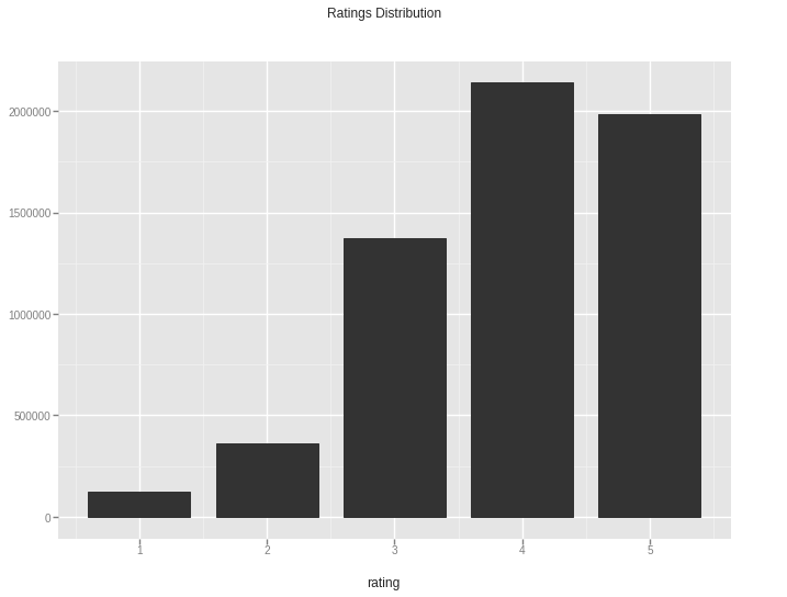
If we look at the distribution of ratings, We can notice that:
-
the values are discrete (1 to 5), but we will deal with them as continuous as we are ok with predicting intermediate values.
-
the data is unbalanced, and most of the ratings are from 3 to 5. (Ideally we should consier the impact of such imbalance on the model)
Train/Test Split
We can look further into the dataset and select books with number of reviews above a certain threshold, or exclude certain records. But for simplicity, we will use the data as is and keep 10% for testing.
from sklearn.model_selection import train_test_split

## split the data to train and test dataframes
train, test = train_test_split(ratings, test_size=0.1)

f"The training and testing data include {len(train), len(test)} records."
'The training and testing data include (5378831, 597648) records.'
Keras Models
As we have our data ready, we can create Keras models to implement the concepts discussed above. We will use the functional API as we need to build multi-input models.
## import keras models, layers and optimizers
from keras.models import Sequential, Model
from keras.layers import Embedding, Flatten, Dense, Dropout, concatenate, multiply, Input
from keras.optimizers import Adam
Using TensorFlow backend.
1- Matrix factorization method
The core of this methods is having:
- users and books embedding layers with the same number of factors.
- user and books bias layers which can be considered as representation of the unique inherent characteristic of each user/book.
We will take the element-wise product of the two embeddings and add the bias terms. The rest is all about experimenting with layers and tuning hyper parameters.
Create model
## define embeddingg size (similar for both users and books)
dim_embedddings = 30
bias = 1

# books
book_input = Input(shape=[1],name='Book')
book_embedding = Embedding(n_books+1, dim_embedddings, name="Book-Embedding")(book_input)
book_bias = Embedding(n_books + 1, bias, name="Book-Bias")(book_input)

# users
user_input = Input(shape=[1],name='User')
user_embedding = Embedding(n_users+1, dim_embedddings, name="User-Embedding")(user_input)
user_bias = Embedding(n_users + 1, bias, name="User-Bias")(user_input)


matrix_product = multiply([book_embedding, user_embedding])
matrix_product = Dropout(0.2)(matrix_product)

input_terms = concatenate([matrix_product, user_bias, book_bias])
input_terms = Flatten()(input_terms)

## add dense layers
dense_1 = Dense(50, activation="relu", name = "Dense1")(input_terms)
dense_1 = Dropout(0.2)(dense_1)
dense_2 = Dense(20, activation="relu", name = "Dense2")(dense_1)
dense_2 = Dropout(0.2)(dense_2)
result = Dense(1, activation='relu', name='Activation')(dense_2)

## define model with 2 inputs and 1 output
model_mf = Model(inputs=[book_input, user_input], outputs=result)

## show model summary
model_mf.summary()
__________________________________________________________________________________________________
Layer (type)                    Output Shape         Param #     Connected to
==================================================================================================
Book (InputLayer)               (None, 1)            0
__________________________________________________________________________________________________
User (InputLayer)               (None, 1)            0
__________________________________________________________________________________________________
Book-Embedding (Embedding)      (None, 1, 30)        300030      Book[0][0]
__________________________________________________________________________________________________
User-Embedding (Embedding)      (None, 1, 30)        1602750     User[0][0]
__________________________________________________________________________________________________
multiply_1 (Multiply)           (None, 1, 30)        0           Book-Embedding[0][0]
                                                                 User-Embedding[0][0]
__________________________________________________________________________________________________
dropout_1 (Dropout)             (None, 1, 30)        0           multiply_1[0][0]
__________________________________________________________________________________________________
User-Bias (Embedding)           (None, 1, 1)         53425       User[0][0]
__________________________________________________________________________________________________
Book-Bias (Embedding)           (None, 1, 1)         10001       Book[0][0]
__________________________________________________________________________________________________
concatenate_1 (Concatenate)     (None, 1, 32)        0           dropout_1[0][0]
                                                                 User-Bias[0][0]
                                                                 Book-Bias[0][0]
__________________________________________________________________________________________________
flatten_1 (Flatten)             (None, 32)           0           concatenate_1[0][0]
__________________________________________________________________________________________________
Dense1 (Dense)                  (None, 50)           1650        flatten_1[0][0]
__________________________________________________________________________________________________
dropout_2 (Dropout)             (None, 50)           0           Dense1[0][0]
__________________________________________________________________________________________________
Dense2 (Dense)                  (None, 20)           1020        dropout_2[0][0]
__________________________________________________________________________________________________
dropout_3 (Dropout)             (None, 20)           0           Dense2[0][0]
__________________________________________________________________________________________________
Activation (Dense)              (None, 1)            21          dropout_3[0][0]
==================================================================================================
Total params: 1,968,897
Trainable params: 1,968,897
Non-trainable params: 0
__________________________________________________________________________________________________
Train model
We will initially train the model for 4 epochs and monitor the loss on the training and validation data.
## specify learning rate (or use the default)
opt_adam = Adam(lr = 0.002)

## compile model
model_mf.compile(optimizer = opt_adam, loss = ['mse'], metrics = ['mean_absolute_error'])

## fit model
history_mf = model_mf.fit([train['user_id'], train['book_id']],
                          train['rating'],
                          batch_size = 256,
                          validation_split = 0.005,
                          epochs = 4,
                          verbose = 0)
## show loss at each epoch
pd.DataFrame(history_mf.history)
| loss | mean_absolute_error | val_loss | val_mean_absolute_error | |
|---|---|---|---|---|
| 0 | 1.108056 | 0.786512 | 0.877477 | 0.746086 |
| 1 | 0.890867 | 0.752475 | 0.874341 | 0.745861 |
| 2 | 0.883530 | 0.748171 | 0.872553 | 0.744265 |
| 3 | 0.874442 | 0.743089 | 0.877095 | 0.746894 |
Interpretation of embedding/bias values
Ideally, if we have trained the model enough to learn about the latent factors of the users/books, the values of the bias or embedding matrices should have a meaning about the underlying characteristics of what they represent. Although this model is preliminary, we will see how we could interpret these values with a good model.
First, we will create a dictionary with the book id and title.
## create a dictionary out of bookid, book original title
books_dict = books.set_index('book_id')['original_title'].to_dict()
Then we will extract the book embedding weights, and we can see it has the expected dimensions.
## get weights of the books embedding matrix
book_embedding_weights = model_mf.layers[2].get_weights()[0]
book_embedding_weights.shape
(10001, 30)
To compress these these vectors into fewer dimensions, we can use Principal Component Analysis(PCA) to reduce the dim_embedddings to three components.
## import PCA
from sklearn.decomposition import PCA

pca = PCA(n_components = 3) ## use 3 components
book_embedding_weights_t = np.transpose(book_embedding_weights) ## pass the transpose of the embedding matrix
book_pca = pca.fit(book_embedding_weights_t) ## fit

## display the resulting matrix dimensions
book_pca.components_.shape
(3, 10001)
We can look at the percentage of variance explained by each of the selected components.
## display the variance explained by the 3 components
book_pca.explained_variance_ratio_
array([0.05605826, 0.04027387, 0.03940241], dtype=float32)
If the variance explained is very low, we might not be able to see a good interpretation. However, for demo purposes, we will just extract the first component/factor that explains the highest percentage of the variance. The array we get can be mapped to the books names as follows.
from operator import itemgetter

## extract first PCA
pca0 = book_pca.components_[0]

## get the value (pca0, book title)
book_comp0 = [(f, books_dict[i]) for f,i in zip(pca0, list(books_dict.keys()))]
If we look at the two extremes on this axis, we will get the following results. Ideally with a good model, we should find the top ten books sharing a certain feature like (genre, movies, etc.), while the lowest ten should be on the opposite side.
I personally couldn’t identify this in the following lists, specially that the variance explained is very low. We we could infer reasons like:
- the model is still not good enough.
- the data requires filtering before building the model.
- I am not familiar with all these books.
- other reasons.
So we can keep tuning the model and we might find a good interpretation for the embedding weights and their PCs.
## books corresponding to the highest values of pca0
sorted(book_comp0, key = itemgetter(0), reverse = True)[:10]
[(0.041030616, 'Marcelo in the Real World'),
 (0.033737715,
  'La increíble y triste historia de la cándida Eréndira y de su abuela desalmada'),
 (0.033430003, 'The Heart of the Matter'),
 (0.031954385, 'Tigers in Red Weather'),
 (0.031844206, 'Inferno'),
 (0.031438835, 'Strange Candy'),
 (0.031019075, 'Going Bovine'),
 (0.03061295, 'Mr Maybe'),
 (0.03044088, 'The Brightest Star in the Sky'),
 (0.029933348, 'The Road to Little Dribbling')]
## books corresponding to the lowest values of pca0
sorted(book_comp0, key = itemgetter(0))[:10]
[(-0.049701463, 'The Reluctant Fundamentalist'),
 (-0.046037737, 'Stolen Prey'),
 (-0.043048386, 'Little Bear'),
 (-0.041676216, 'Frog and Toad All Year'),
 (-0.04117827, 'The Complete Works'),
 (-0.039489016, 'For Love of Evil'),
 (-0.037475895, "I've Got You Under My Skin"),
 (-0.035478182, 'Анна Каренина'),
 (-0.035430357, 'A Thousand Boy Kisses'),
 (-0.03501414, 'The Exploits of Sherlock Holmes')]
2- Tabular data method
In this method, we will just have users and books embedding layers that can have different dimensions. We will concatenate them together as if we have a table with dim_embedding_user+dim_embedding_book features. Then we can add dense layers, or even use these weights as features with other algorithms.
Define model
## define the number of latent factors (can be different for the users and books)
dim_embedding_user = 50
dim_embedding_book = 50

## book embedding
book_input= Input(shape=[1], name='Book')
book_embedding = Embedding(n_books + 1, dim_embedding_book, name='Book-Embedding')(book_input)
book_vec = Flatten(name='Book-Flatten')(book_embedding)
book_vec = Dropout(0.2)(book_vec)

## user embedding
user_input = Input(shape=[1], name='User')
user_embedding = Embedding(n_users + 1, dim_embedding_user, name ='User-Embedding')(user_input)
user_vec = Flatten(name ='User-Flatten')(user_embedding)
user_vec = Dropout(0.2)(user_vec)

## concatenate flattened values
concat = concatenate([book_vec, user_vec])
concat_dropout = Dropout(0.2)(concat)

## add dense layer (can try more)
dense_1 = Dense(20, name ='Fully-Connected1', activation='relu')(concat)

## define output (can try sigmoid instead of relu)
result = Dense(1, activation ='relu',name ='Activation')(dense_1)

## define model with 2 inputs and 1 output
model_tabular = Model([user_input, book_input], result)

## show model summary
model_tabular.summary()
__________________________________________________________________________________________________
Layer (type)                    Output Shape         Param #     Connected to
==================================================================================================
Book (InputLayer)               (None, 1)            0
__________________________________________________________________________________________________
User (InputLayer)               (None, 1)            0
__________________________________________________________________________________________________
Book-Embedding (Embedding)      (None, 1, 50)        500050      Book[0][0]
__________________________________________________________________________________________________
User-Embedding (Embedding)      (None, 1, 50)        2671250     User[0][0]
__________________________________________________________________________________________________
Book-Flatten (Flatten)          (None, 50)           0           Book-Embedding[0][0]
__________________________________________________________________________________________________
User-Flatten (Flatten)          (None, 50)           0           User-Embedding[0][0]
__________________________________________________________________________________________________
dropout_4 (Dropout)             (None, 50)           0           Book-Flatten[0][0]
__________________________________________________________________________________________________
dropout_5 (Dropout)             (None, 50)           0           User-Flatten[0][0]
__________________________________________________________________________________________________
concatenate_2 (Concatenate)     (None, 100)          0           dropout_4[0][0]
                                                                 dropout_5[0][0]
__________________________________________________________________________________________________
Fully-Connected1 (Dense)        (None, 20)           2020        concatenate_2[0][0]
__________________________________________________________________________________________________
Activation (Dense)              (None, 1)            21          Fully-Connected1[0][0]
==================================================================================================
Total params: 3,173,341
Trainable params: 3,173,341
Non-trainable params: 0
__________________________________________________________________________________________________
Train model
## specify learning rate (or use the default by specifying optimizer = 'adam')
opt_adam = Adam(lr = 0.002)

## compile model
model_tabular.compile(optimizer= opt_adam, loss= ['mse'], metrics=['mean_absolute_error'])

## fit model
history_tabular = model_tabular.fit([train['user_id'], train['book_id']],
                                    train['rating'],
                                    batch_size = 256,
                                    validation_split = 0.005,
                                    epochs = 4,
                                    verbose = 0)
This model performs better that the first one after 4 epochs. Part of the experimentation is to train both for more epochs, tune the hyper parameters or modify the architecture.
## show loss at each epoch
pd.DataFrame(history_tabular.history)
| loss | mean_absolute_error | val_loss | val_mean_absolute_error | |
|---|---|---|---|---|
| 0 | 0.819832 | 0.701705 | 0.728423 | 0.657826 |
| 1 | 0.721092 | 0.661850 | 0.703210 | 0.649271 |
| 2 | 0.693019 | 0.645749 | 0.688836 | 0.636335 |
| 3 | 0.674404 | 0.635130 | 0.681535 | 0.645501 |
Predict ratings of test data
If we want to check the model, we can use the test data which gives mse close to the validation loss.
## import libraries
from sklearn.metrics import mean_absolute_error, mean_squared_error

## define a function to return arrays in the required form
def get_array(series):
    return np.array([[element] for element in series])

## predict on test data
predictions = model_tabular.predict([get_array(test['user_id']), get_array(test['book_id'])])

f'mean squared error on test data is {mean_squared_error(test["rating"], predictions)}'
'mean squared error on test data is 0.6897965023610527'
3- Other methods
Although we saw preliminary models we could get the idea behind each of the methods and we have a starting point to experiment more. There’s also another approach which almost combines both methods. It was published in a paper entitled Neural Collaborative Filtering. I haven’t experimented with it but I thought it was worth mentioning as we discuss similar methods.
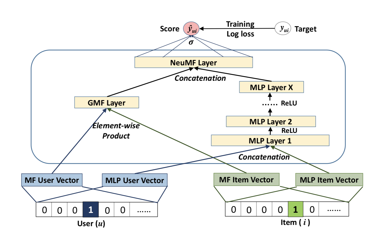 Source: Neural Collaborative Filtering, Xiangnan He, Lizi Liao, Hanwang Zhang, Liqiang Nie, Xia Hu, and Tat-Seng Chua.
fast.ai Model
Also fast.ai library provides dedicated classes and fucntions for collaborative filtering problems built on top on PyTorch. It includes more advanced options by default like using the The 1cycle policy and other settings. The following few lines will implement the matrix factorization method. But I will not discuss further details in the post.
%%script false

## import fast.ai modules
from fastai.collab import *
from fastai.tabular import *

## define user/item column names in the training data
user, item = 'user_id','book_id'

## find learning rate
learn.lr_find()
learn.recorder.plot()

## create data bunch
data = CollabDataBunch.from_df(train, seed=42)

## specify the sigmoid limits
y_range = [0, 5.5]

## define learner
learn = collab_learner(data, n_factors = 50, y_range = y_range)

## fit the model and monitor mse
learn.fit_one_cycle(3, 0.01)
Conclusion
In this post we had an overview about the use of embeddings for matrix factorization and feature creation. We trained preliminary models in Keras to understand the possible architectures for the two mentioned methods. We also had an overview about the implementation in fast.ai library. It is worth mentioning that in practice I would take more time to inspect the dataset and might modify it unless it is one with a benchmark. I could also look into other metrics or specific groups which were less represented. But the main purpose of the post was to go over the main ideas and see code examples as a first step of experimentation.
References and Readings
- Practical Deep Learning for Coders Lesson 4: NLP, Tabular data, Collaborative filtering, Embeddings, Jeremy Howard, fast.ai
- Understanding Latent Style, Erin Boyle and Jana Beck, StitchFix
- Neural Collaborative Filtering, Xiangnan He, Lizi Liao, Hanwang Zhang, Liqiang Nie, Xia Hu, and Tat-Seng Chua.