In the previous post, we had an overview about text pre-processing in keras. In this post we will use a real dataset from the Toxic Comment Classification Challenge on Kaggle which solves a multi-label classification problem.
In this competition, it was required to build a model that’s “capable of detecting different types of toxicity like threats, obscenity, insults, and identity-based hate”. The dataset includes thousands of comments from Wikipedia’s talk page edits and each comment can have more than one tag.
Dataset Exploration
First of all let’s load our train and test data.
## load libraries
library(keras)
library(tidyverse)
library(here)
## read train and test data
train_data <- read_csv(here("static/data/", "toxic_comments/train.csv"))
test_data <- read_csv(here("static/data/", "toxic_comments/test.csv"))Training data columns
We can see that the training dataframe includes columns with the comment id, text then six target tags.
names(train_data)## [1] "id" "comment_text" "toxic" "severe_toxic"
## [5] "obscene" "threat" "insult" "identity_hate"Target labels distribution
Notice that:
the way the target labels are given (six columns with binary values) is good because that’s what we need to give to our network.
it is possible to have multiple tags = 1 for the same comment, since a comment can be tagged, for instance, as toxic and threat at the same time.
If we look at the percentage of comments under each tag, we can see the following distribution:
| toxic | severe_toxic | obscene | threat | insult | identity_hate |
|---|---|---|---|---|---|
| 9.58% | 1.000% | 5.29% | 0.300% | 4.94% | 0.880% |
Data Processing
Before defining our model, we need to prepare the text and targets in the proper format.
Process comments text
As we understood the structure of our data, we can start to process the text. We learned in part one that we can represent the words in our vocabulary in a compact form using word embeddings before adding any other layers. In the next sections we will do the tokenization and padding steps to create our sequences.
Note that it is possible to make extra pre-processing, by normalizing or cleaning the text, but in some cases the typos add a useful noise that helps in generalization. This is part of experimentation while trying to improve the acccuracy of the model.
Tokenize comments text
Given that the text we have includes tens or hundreds of thousands of unique words, we need to limit this number. So we will initialize a tokenizer and use vocab_size to keep the most frequent 20000 words.
Note that you should only use the comment_text from the train data because ideally you won’t have the test data till the end. And you shouldn’t learn anything from it anyways.
## define vocab size (this is parameter to play with)
vocab_size = 20000

tokenizer <- text_tokenizer(num_words = vocab_size) %>%
  fit_text_tokenizer(train_data$comment_text)
Create sequences from tokens
Now we can use the tokenizer to create sequences from both the train and test data.
## create sequances
train_seq <- texts_to_sequences(tokenizer, train_data$comment_text)
test_seq <- texts_to_sequences(tokenizer, test_data$comment_text)
You can see how the comments turned into sequences as shown in the following example:
train_data$comment_text[1]## [1] "Explanation\nWhy the edits made under my username Hardcore Metallica Fan were reverted? They weren't vandalisms, just closure on some GAs after I voted at New York Dolls FAC. And please don't remove the template from the talk page since I'm retired now.89.205.38.27"turned into:
train_seq[1]## [[1]]
## [1] 688 75 1 126 130 177 29 672 4511 12052 1116
## [12] 86 331 51 2278 11448 50 6864 15 60 2756 148
## [23] 7 2937 34 117 1221 15190 2825 4 45 59 244
## [34] 1 365 31 1 38 27 143 73 3462 89 3085
## [45] 4583 2273 985Pad sequences to unify the length
As we know the lengths of the comments are not equal, we need to pad them with zeros to unify their length. We can decide the maximum length based on the data we have.
So let’s look at a histogram of the comments lengths after using the tokenizer.
Training data comments length
## calculate training comments lengths
comment_length <- train_seq %>%
  map(~ str_split(.x, pattern = " ", simplify = TRUE)) %>%
  map_int(length)

## plot comments length distribution
data_frame(comment_length = comment_length)%>%
  ggplot(aes(comment_length))+
  geom_histogram(binwidth = 20)+
  theme_minimal()+
  ggtitle("Training data comments length distribution")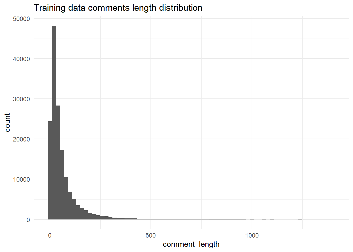
Padding
For this experiment, I will pick 200 as maximum length. This is one of the values you can experiment with.
## define max_len
max_len = 200

## pad sequence
x_train <- pad_sequences(train_seq, maxlen = max_len, padding = "post")
x_test <- pad_sequences(test_seq, maxlen = max_len, padding = "post")
prepare targets columns
since keras models take matrices, we will select the target columns and convert to a matrix as follows:
## extract targets columns and convert to matrix
y_train <- train_data %>%
  select(toxic:identity_hate) %>%
  as.matrix()
keras model
Now let’s define a simple sequential model and test is.
Define the model
Note that in the following model:
the embedding layer come first. It takes the
input_dimwhich is the number of words/features (herevocab_size) and theoutput_dimwhich is the embedding vector size. It is common to take the embeddings size as 50, 100 or more but the bigger the value the more trainable parameters. So it will take more time.a global average pooling layer is used to convert the 2D output from the embedding layer to 1D that could be fed to the subsequent layers. you can also try global max pooling.
the output should have six units because we have six tags.
the
sigmoidactivation suits the problem here because it allows two or more tags with high probabilities simultaneously, which suits our problem.in between the pooling layer and the output we have a dense layer for simplicity, and we can experiment with the number of units.
## define embedding size
emd_size = 64

## define model
model <- keras_model_sequential() %>%
  layer_embedding(input_dim = vocab_size, output_dim = emd_size) %>%
  layer_global_average_pooling_1d() %>%
  layer_dense(units = 32, activation = "relu") %>%
  layer_dense(units = 6, activation = "sigmoid")
Now you can see a summary of the model as follows:
summary(model)## ___________________________________________________________________________
## Layer (type) Output Shape Param #
## ===========================================================================
## embedding_1 (Embedding) (None, None, 64) 1280000
## ___________________________________________________________________________
## global_average_pooling1d_1 (Glob (None, 64) 0
## ___________________________________________________________________________
## dense_1 (Dense) (None, 32) 2080
## ___________________________________________________________________________
## dense_2 (Dense) (None, 6) 198
## ===========================================================================
## Total params: 1,282,278
## Trainable params: 1,282,278
## Non-trainable params: 0
## ___________________________________________________________________________Compile the model
After that, you can compile the model. Note that:
the
optimizeradamis picked as it is known to work well in such problems.the
lossisbinary_crossentropybecause with multi-label classification, it is as if you have a binary classification problem but on six labels.
## specify model optimizer, loss and metrics
model %>% compile(
  optimizer = 'adam',
  loss = 'binary_crossentropy',
  metrics = 'accuracy'
)
Fit the model
After compiling the model, we are ready to fit it. We can save the model results in a list (history here).
Note that:
We can specify a portion of the data for validation using the
validation_splitparameter.We can start with less
epochs, however I picked 16 for demo purposes.
history <- model %>%
  fit(x_train,
      y_train,
      epochs = 16,
      batch_size = 64,
      validation_split = 0.05,
      verbose = 0)

# saveRDS(history, here("static/data/", "toxic_comments/history_seq.rds"))
If we plot the history, we can see the loss and accuracy over the 16 epochs. Note that:
the two curves diverge and the validation accuracy plateaus after 4 or 5 epochs. So the best model might be obtained around the epoch #5.
the accuracy is not bad given the simple model we built. So there could be a room for higher accuracy with more sophisticated models.
You can try and train the model from scratch for 4 or 5 epochs. Another option is to save the best model while training for 16 epochs (we will talk about this in another post).
plot(history)+
  theme_minimal()+
  ggtitle("Loss and Accuracy Curves")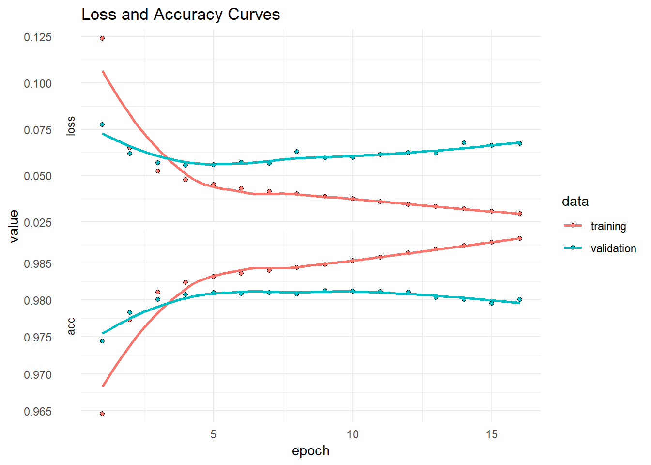
Predict test labels
Once you have the final model, you can predict the test labels.
## predict on test data
predicted_prob <- predict_proba(model, x_test)
If you want to submit the result to Kaggle, you need to create a dataframe with ids and predictions.
## join ids and predictions
y_test <- as_data_frame(predicted_prob)
names(y_test) <- names(train_data)[3:8] ## labels names
y_test <- add_column(y_test, id = test_data$id, .before = 1) ## add id column
This simple model could get around 0.96 on the Private Score, which is not bad but still far from the mid-level submissions. It is just a good start, but there are other models that would perform better. In the next post we will try different types of architectures and play with other options in keras.