Almost a year ago I wrote about my My First Steps into The World of Tidy Eval. At the end I tweeted asking Hadley Wickham and Lionel Henrey whether ggplot2 was compatible with the tidy eval, They said that it was on the todo list.
Finally, ggplot2 3.0.0 got released last week with the support of tidy eval, so I thought it was time to write about it!
ggplot2 3.0.0 now on CRAN — https://t.co/m8fSDaaSbu 🎉 Headline features are tidy eval, sf support, position_dodge2(), & viridis. Huge thanks to all 300+ contributors to this release, and particularly to @ClausWilke, @kara_woo, @_lionelhenry and @thomasp85 pic.twitter.com/igb9k0Z89C
— Hadley Wickham (@hadleywickham) July 4, 2018
In this post, I will go over the traditional ways of using ggplot2 then I will highlight some cases, in which tidy eval solves problems and provides more flexibility.
Dataset
In all the following examples We will use a simple dataset, which is tips from reshape2 package. The dataset contains information about tips received by a waiter over a period of a few months. We will add a new column with tip_percent to use in our plots.
## Load packages
library(reshape2)
library(tidyverse)
## add a new column with tip_percent
tips <- tips %>%
mutate(tip_percent = tip/total_bill)
as_tibble(tips)# A tibble: 244 x 8
total_bill tip sex smoker day time size tip_percent
<dbl> <dbl> <fct> <fct> <fct> <fct> <int> <dbl>
1 17.0 1.01 Female No Sun Dinner 2 0.0594
2 10.3 1.66 Male No Sun Dinner 3 0.161
3 21.0 3.5 Male No Sun Dinner 3 0.167
4 23.7 3.31 Male No Sun Dinner 2 0.140
5 24.6 3.61 Female No Sun Dinner 4 0.147
6 25.3 4.71 Male No Sun Dinner 4 0.186
7 8.77 2 Male No Sun Dinner 2 0.228
8 26.9 3.12 Male No Sun Dinner 4 0.116
9 15.0 1.96 Male No Sun Dinner 2 0.130
10 14.8 3.23 Male No Sun Dinner 2 0.219
# ... with 234 more rowsggplot2 the common way
aes()
The common way of using ggplot2 functions, and the first example most people try is using Non standard Evaluation (NSE), by passing variable names unquoted. For instance if you want to plot tip_percent versus total_bill you could simply write the following chunk of code.
ggplot(tips, aes(x = total_bill,
                 y = tip_percent,
                 alpha = 0.5))+
  geom_point()+
  theme_minimal()+
  guides(alpha = FALSE)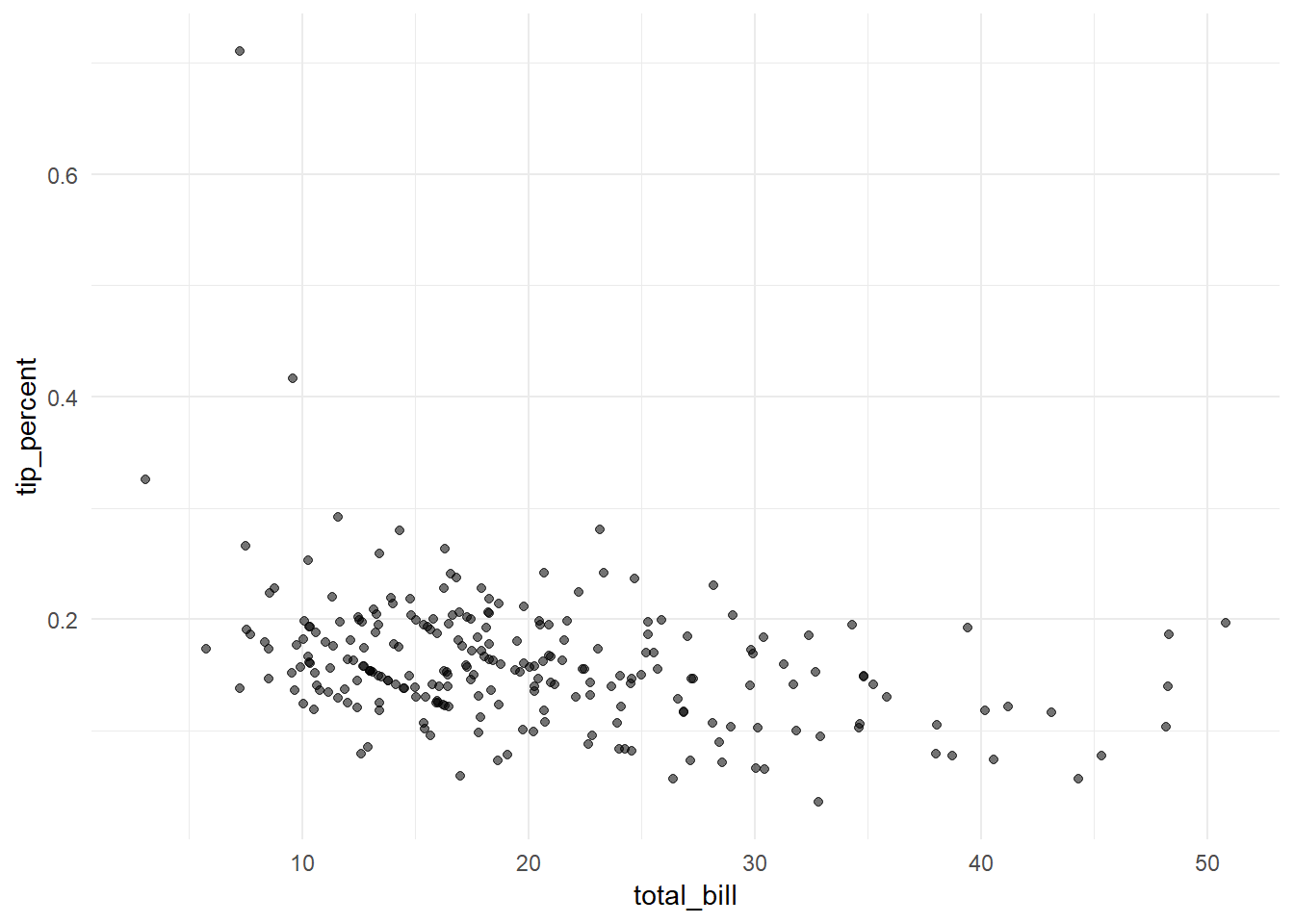
aes_string()
Another way is using aes_string() instead of aes(). In this case, you will need to pass column names quoted as follows, which will give the same result.
ggplot(tips, aes_string(x = "total_bill",
                 y = "tip_percent",
                 alpha = 0.5))+
  geom_point()+
  theme_minimal()+
  guides(alpha = FALSE)
This version could be helpful when you want to pass variables to ggplot2 functions. For instance, you can handle a scenario, when you have pre-defined variables to use, or in case you take the variable names from a user through an interface. The following examples will work fine and give the same result.
## define variables
x_var <- "total_bill"
y_var <- "tip_percent"
alpha_var <- 0.5

ggplot(tips, aes_string(x = x_var,
                 y = y_var,
                 alpha = alpha_var))+
  geom_point()+
  theme_minimal()+
  guides(alpha = FALSE)
And usually the use case for this, is the need to write a reusable function that wraps several ggplot2 layers to work with whatever variables passed to it. For example, you can wrap the previous chunk in a function as follows
plot_points <- function(x, y, alpha){
  ggplot(tips, aes_string(x = x, y = y, alpha = alpha))+
  geom_point()+
  theme_minimal()+
  guides(alpha = FALSE)
}
Then you can either pass column names directly or the variable names.
## pass column names directly
plot_points(x = "total_bill",
            y = "tip_percent",
            alpha = 0.5)

## pass variable names
plot_points(x = x_var,
            y = y_var,
            alpha = alpha_var)
And you can reuse the function to create similar plots with different variables. For instance tip on the y-axis instead of tip_percent
## plot tip vs. total_bill
plot_points(x = "total_bill",
            y = "tip",
            alpha = 0.5)
ggplot2 the tidy eval way
The previous options are good and valid in many cases, but there are some limitations. For instance, you cannot create a function and pass column names unquoted as follows.
plot_points2 <- function(x, y, alpha){
  ggplot(tips, aes(x = x, y = y, alpha = alpha))+
    geom_point()+
    theme_minimal()+
    guides(alpha = FALSE)
}

## invalid way
plot_points2(x = total_bill,
             y = tip_percent,
             alpha = 0.5)
This will just break and gives an error like:
Error in FUN(X[[i]], ...) : object 'total_bill' not found
Previously there was no straightforward way to handle this, but with tidy eval it became possible and easy.
Unquoted column names / NSE
You can use enquo() and the bang bang operator !! to create a function like plot_points_tidyeval_01() which takes the column names unquoted, and it will work properly.
plot_points_tidyeval_01 <- function(x, y, alpha){

  x_var <- enquo(x)
  y_var <- enquo(y)

  ggplot(tips, aes(x = !!x_var, y = !!y_var, alpha = alpha))+
    geom_point()+
    theme_minimal()+
    guides(alpha = FALSE)
}

## pass column names unquoted
plot_points_tidyeval_01(x = total_bill,
                        y = tip_percent,
                        alpha = 0.5)
You might still see this as a simple use case that could be handled by aes_string(). But there are more things you can do, like variable facets.
Variable Facets
Suppose that you wanted to define a variable facet, you wouldn’t have this flexibility even with aes_string(). But now you can implement it as follows.
Notice that vars() is a new helper inside facet_grid instead of the ~.
plot_points_tidyeval_02 <- function(x, y, alpha, facet){

  x_var <- enquo(x)
  y_var <- enquo(y)
  facet_var <- enquo(facet)

  ggplot(tips, aes(x = !!x_var, y = !!y_var, alpha = alpha))+
    geom_point()+
    theme_minimal()+
    guides(alpha = FALSE)+
    facet_grid(cols = vars(!!facet_var))}
So you can pass sex to the facet variable in the plot_points_tidyeval_02() function.
## use sex for facet
plot_points_tidyeval_02(x = total_bill,
                        y = tip_percent,
                        alpha = 0.5,
                        facet = sex)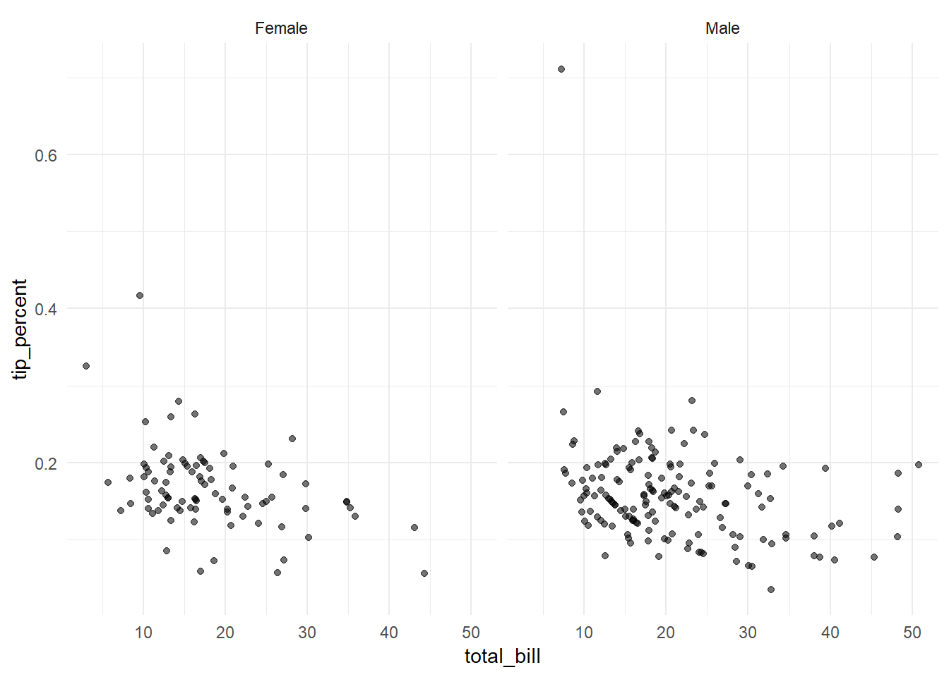
or a different variable like day
## use day for facet
plot_points_tidyeval_02(x = total_bill,
                        y = tip_percent,
                        alpha = 0.5,
                        facet = day)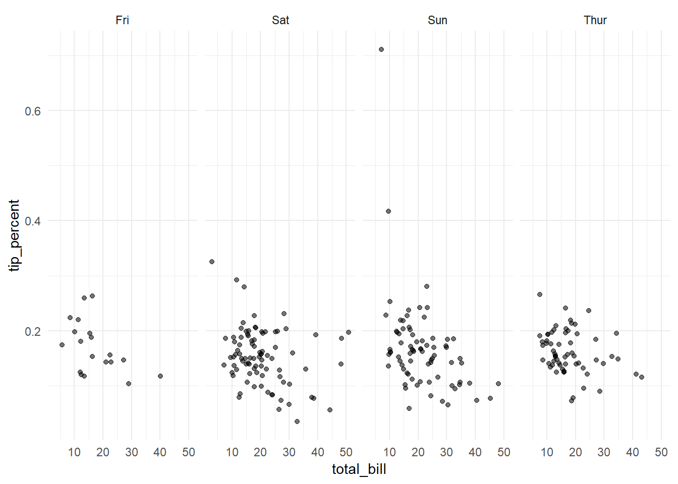
You can even use the dots ... to have more flexibility and allow the function to take more than one variable for faceting. You can pass the dots ... directly to vars() inside facet_wrap() as follows.
plot_points_tidyeval_03 <- function(x, y, alpha, ...){

  x_var <- enquo(x)
  y_var <- enquo(y)

  ggplot(tips, aes(x = !!x_var, y = !!y_var, alpha = alpha))+
    geom_point()+
    theme_minimal()+
    guides(alpha = FALSE)+
    facet_wrap(vars(...), nrow = 2)
}


## use both sex and day for facets
plot_points_tidyeval_03(x = total_bill,
                        y = tip_percent,
                        alpha = 0.5,
                        sex, day)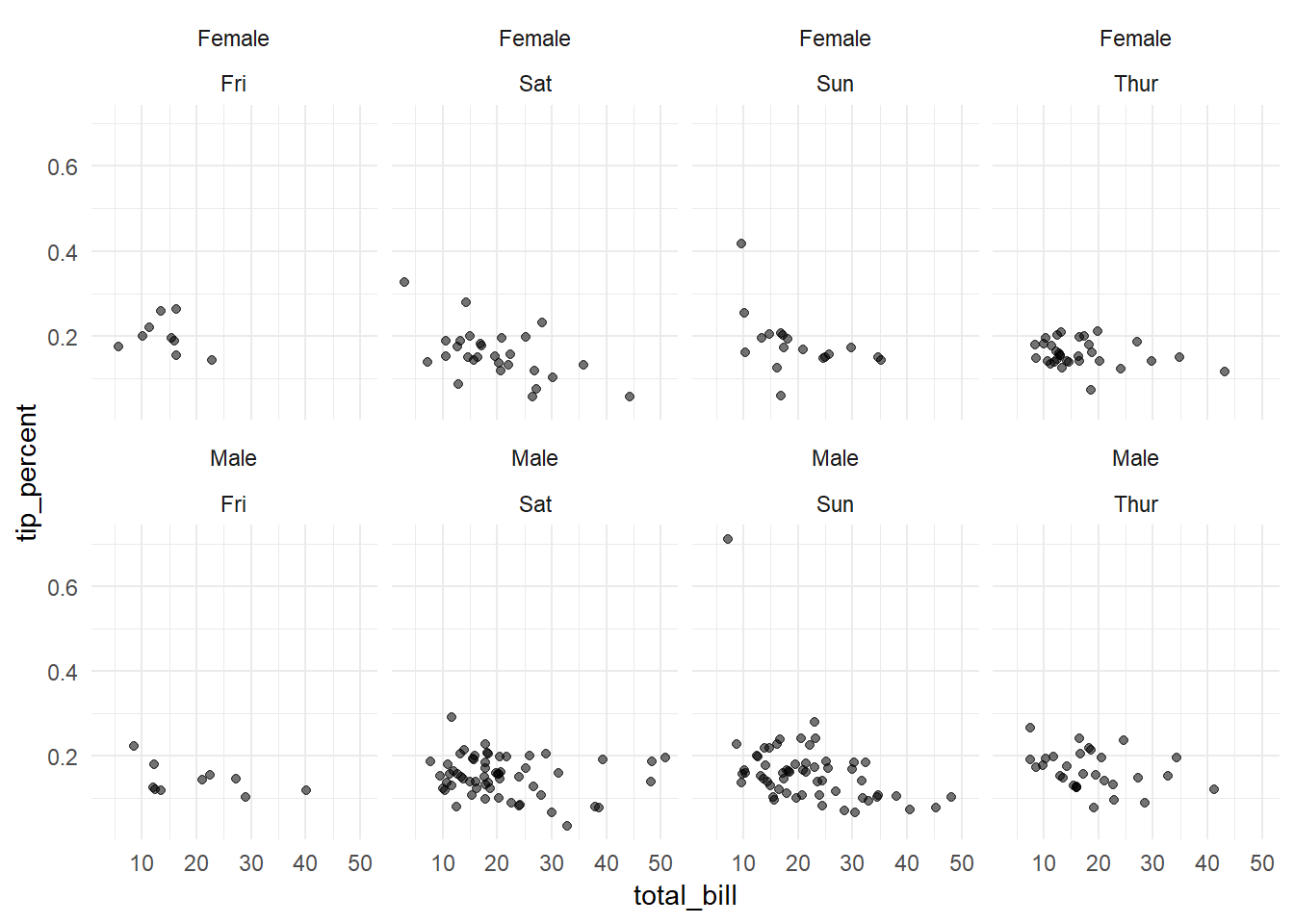
In Conclusion
tidy eval with ggplot2 offers new options and more capabilities. It solves problems people used to struggle with and gives a higher level of flexibilty in writing functions and programming. I just covered a couple of options in this post, but I am sure I will discover more stuff and hopefully write about them later.