Everyday statisticians, analysts and data enthusiasts perform data analysis for different purposes. But when it comes to presenting analyses to wider audience, the good work is not the complex one with big words. It is the one that highlights interesting relations, answers business questions or predict outcomes, and explain all that in the simplest way through data visualization or simple concepts. So if one throws numbers, model coefficients and complex graphs to impress the audience, it might fireback if the audience are not familiar with a certain concept.

For example, logistic regression is one of the models that is not intuitively understood by non-stats. To be frank, even for me, the first time I learnt about it, I was not so confident about interpreting the results. It took me sometime to go through the math and work out some examples before I grasped it. So if you go to a business meeting, or present results of a clinical trial to help your audience take decisions, talking about log odds ratio will probably make you lose them immediately. People are more familar with probabilities and odds, so it is recommended to highlight these values.

In this post, I will show examples on interpreting logistic regression coefficients and try to highlight the values to be communicated with others in an intuitive way. I will use a sample data set, taken from idre UCLA, where similar examples where discussed. The dataset has observations for 200 students and we are interested in the variable hon as the outcome, which indicates if a student is in an honors class or not.

What The Audience Would Like To Hear

In principle, audience would like to hear values that can be interpreted instantaneously in their minds, values they can compare easily to make judgement. If you have results based on logistic regression models, you don’t want people to struggle with converting values in their minds.

So let’s take the first example that will be discussed in detail in the Examples section. For now, we will start with the end, i.e. the final values to be presented to audience from different backgrounds and to non-quants.

In this example, we use a binary predictor variable female to predict whether a student is in an honors class hon or not. Most probably, audience will be interested in values such as:

Propability that a male/female goes to an honors class.
odds of male/femal being in an honors class.
The relative change in odds of being in an honors class, when going from male to female.

These values are not given directly by the logistic regression model, but we can calculate and highlight them.

Propabilities

Any one with any background will be able to get that the probability of a female being in honors class 0.2936, is higher than the probability of a male being in honors class 0.1868.

Odds

And if someone is not even familiar with probabilities, the odds are straightforward. Anyone can get the following statements and compare easily:

for every 23 male in honors class, 100 will be in a non-honors class*
for every 42 female in honors class, 100 will be in a non-honors class*

It will also be easy for them to see that going from male to female increases the odds by around 82%*, which is the odds ratio.

(*NOTE: values are rounded since we are dealing with humans not things to be divided, the accurate values are listed in the examples)

By highlighting these values, the audience will be able to process the results of the analysis easily and see the value in it because it will help them judge different options, treatments, categories, campaigns..etc. And consequently enable them to make data-driven decisions. Surely, with more predictors and more interactions, it gets more complex, but the key is to express the results in simple statements using probabilities and odds.

So this was what we can extract from our model, but what about the model itself? , what does it represent? and how can we interpret the coefficients and convert them to odds and propabilities?

What You Need To Know About Logistic Regression

If you want to be work with logistic regression models and present results in a simple way, you need to be confident with the main concepts. The following sections focus on the basics and give simple examples with categorical and continuous predictors.

Background (Propabilities, Odds, And Odds Ratio)

Logistic regression models the logit-transformed probability as a linear relationship with the predictor variables. It converts probabilities into the whole real line, as it is usually hard to model a variable with a restricted range. So we go from probability to logit as follows:

Probability

{% raw %}

{% endraw %}

Odds

{% raw %}

{% endraw %}

Log Odds

{% raw %}

{% endraw %}

Examples

At the begining, we mentioned a simple logistic regression example with a categorical predictor, and highlighted the values of interest for general audience. let’s see how we get these values from the model and how to interpret more complex ones. We will also see another example with a continuous predictor variable.

Single Categorical Predictor Variable

If we fit a model with hon as the outcome and female as the predictor:

{% raw %}

{% endraw %}

              Estimate Std. Error   z value     Pr(>|z|)
(Intercept) -1.4708517  0.2689554 -5.468756 4.532047e-08
female       0.5927822  0.3414293  1.736178 8.253231e-02

We can interpret the coefficients and even convert them to probabilities.

Intercept: is the log odds of male being in an honor class (since male is the reference group, female=0)

We can get the odds by exponentiating this value then we can calculate the probability of male being in an honor. Here, we notice that the odds is the value highlighted earlier as 23 to 100 and the probability is the one calculated and shown to the audience.

             log_odds      odds         p
(Intercept) -1.470852 0.2297297 0.1868132

female coefficient: is the log of odds ratio between the female group and male group (or the difference in log odds since log(x)-log(y)=log(x/y))

We can see that the odds ratio is around 1.81 which indicates an increase in the odds by around 81% by going from male to female. This is close to the approximated value highlighted earlier when 42/23 was considered.

       log_odds_ratio odds_ratio         p
female      0.5927822   1.809015 0.6440033

Single Continuous Predictor Variable

Now if we fit a model with hon as the outcome and math as the predictor:

{% raw %}

{% endraw %}

              Estimate Std. Error   z value     Pr(>|z|)
(Intercept) -9.7939421 1.48174484 -6.609736 3.850061e-11
math         0.1563404 0.02560948  6.104784 1.029399e-09

We can interpret the coefficients as follows:

Intercept: is the log odds of a student with a math score of zero being in an honors class

We can see that the odds/probability is very low because a math score of zero is very low, it actually does not exist in the dataset. So this is a hypothetical value and that’s why a very low probability is reasonable.

             log_odds         odds            p
(Intercept) -9.793942 5.578854e-05 5.578543e-05

math coeffiecent: the difference in the log odds (or the expected change in log odds for a one-unit increase in the math score)

     log_odds_diff odds_ratio         p
math     0.1563404   1.169224 0.5390057

To be more confident with this interpretation, let’s calculate the log odds at two math scores according to the equation:

{% raw %}

{% endraw %}

{% raw %}

{% endraw %}

{% raw %}

{% endraw %}

{% raw %}

{% endraw %}

We can see the calculated difference in log odds is equal to the math coefficient obtained by the model.

If we exponentiate the difference in log odds, we get the odds ratio (since logarithm converts division to subtraction.). Here the value is 1.1692241 so we can say that we can expect about 17% increase in the odds of being in an honors class for a one-unit increase in math score.

Note that:

The percentage increase in odds does not depend on the value at which math is held.
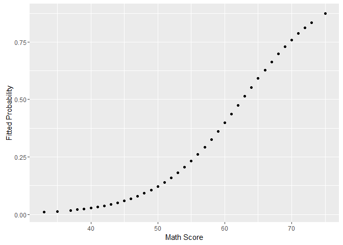
The difference in probabilities is not the same at low, medium, and high values of math score, because the relationship between math and probability is not linear. We can see that if we plot the fitted values from the model versus math. So in case you highlight probabilities in a presentation, you need to make sure your audience get this point. You can give them examples at different ranges, or in the range of interest for them.

So these were the highlights of logistic regression. If you grasp the concept and get confident about it, you will be able to interpret and explain it to others. But make sure you know your audience, and give them what they are interested in the simplest way.